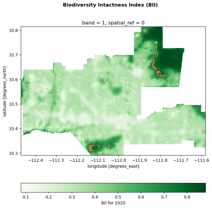
Phoenix Biodoversity Intactness

R
MEDS
data-viz
Geospatial
Author
Affiliation

Joshua Ferrer-Lozano

Master of Environmental Data Science

Published

12-05-2025

Biodiversity Intactness Index Change in Phoenix, AZ

Author : Joshua Ferrer-Lozano Date: 12/5/2025

You can access the full analysis of the project in this Github repository

About

Purpose

This notebook investigates changes in the Biodiversity Intactness Index (BII) in the Phoenix subdivision between 2017 and 2020. The goal is to understand how rapid urban expansion has affected biodiversity.

Highlights

  • Imported and explored BII raster datasets (2017, 2020) from the Microsoft Planetary Computer.
  • Clipped rasters to the Phoenix subdivision shapefile.
  • Calculated the percentage of area with BII ≥ 0.75 for both years.
  • Visualized areas of biodiversity loss between 2017 and 2020.

About the Data

  • BII Time Series (2017, 2020): Global 100m projections of biodiversity intactness, accessed via Microsoft Planetary Computer STAC catalog.
  • Phoenix Subdivision Shapefile: Census County Subdivision shapefiles for Arizona, used to define the study area.
  • Contextual Data: Optional basemap tiles from contextily for geographic context.

References

  • Levitt, Z., & Eng, J. (2021). Where America’s developed areas are growing: ‘Way off into the horizon’. The Washington Post. https://www.washingtonpost.com/nation/interactive/2021/land-development-urban-growth-maps/
  • Gassert, F., Mazzarello, J., & Hyde, S. (2022). Global 100m Projections of Biodiversity Intactness for the years 2017-2020 [Technical Whitepaper]. https://ai4edatasetspublicassets.blob.core.windows.net/assets/pdfs/io-biodiversity/Biodiversity_Intactness_whitepaper.pdf
  • Microsoft Planetary Computer, STAC Catalog. Biodiversity Intactness (‘io-biodiversity’). [Dataset]. https://planetarycomputer.microsoft.com/dataset/io-biodiversity Accessed 6 December 2023.

Import Libraries

# Load in Libraries

import os
import pandas as pd
import geopandas as gpd
import matplotlib.pyplot as plt
import matplotlib.patches as patch

# geospatial libraries
import xarray as xr
import rioxarray as rio
from shapely.geometry import box

# Planetary Computer Access
import contextily as ctx
import planetary_computer

# Check python environment
import sys
print(sys.executable)

from pystac_client import Client

c:\Users\joshu\.conda\envs\eds220-env\python.exe

Access Planetary Computer STAC Catalog: io-biodiversity collection

# Connect to the Planetary Computer STAC API
catalog = Client.open(
    "https://planetarycomputer.microsoft.com/api/stac/v1",
    modifier=planetary_computer.sign_inplace,
)

# Exploring catalog metadata
print('Title', catalog.title)


# Pull out the io_biodiversity collection
io_collection = catalog.get_child('io_biodiversity')
print(io_collection)
Title Microsoft Planetary Computer STAC API
None

Define our parameters


# Temporal range of interest (2017–2020 drought period)
time_range = '2017-01-01/2020-01-01'

# Bounding box for Phoenix subdivision
bbox = [-112.826843, 32.974108, -111.184387, 33.863574]

# Get items from search
search = catalog.search(
    collections = ['io-biodiversity'],
    bbox = bbox,
    datetime = time_range)

# Retrieve items
items = search.item_collection()
print(len(items))
4

Select 2017 and 2020 Raster


# Create a lookup table
lookup = {int(item.properties["start_datetime"][:4]): item for item in items} # year is available inside start_datetime not datetime 

# Store 2017 and 2020 raster
phoenix_2017 = lookup[2017]
phoenix_2020 = lookup[2020]

Arizona Data

# Import Arizona Census Subdivision data

# display all columns when looking at dataframes
pd.set_option("display.max.columns", None)

arizona_fp = os.path.join('data','tl_2022_04_cousub','tl_2022_04_cousub.shp')
arizona = gpd.read_file(arizona_fp)

# preliminary exploration
arizona.head(5)
STATEFP COUNTYFP COUSUBFP COUSUBNS GEOID NAME NAMELSAD LSAD CLASSFP MTFCC CNECTAFP NECTAFP NCTADVFP FUNCSTAT ALAND AWATER INTPTLAT INTPTLON geometry
0 04 005 91198 01934931 0400591198 Flagstaff Flagstaff CCD 22 Z5 G4040 None None None S 12231052883 44653332 +35.1066114 -111.3662497 POLYGON ((-112.13370 35.85596, -112.13368 35.8...
1 04 005 91838 01934953 0400591838 Kaibab Plateau Kaibab Plateau CCD 22 Z5 G4040 None None None S 7228864534 29327221 +36.5991097 -112.1368033 POLYGON ((-112.66039 36.53941, -112.66033 36.5...
2 04 005 91683 01934950 0400591683 Hualapai Hualapai CCD 22 Z5 G4040 None None None S 2342313339 3772690 +35.9271665 -113.1170408 POLYGON ((-113.35416 36.04097, -113.35416 36.0...
3 04 023 92295 01934961 0402392295 Nogales Nogales CCD 22 Z5 G4040 None None None S 1762322938 2382710 +31.4956020 -111.0171332 POLYGON ((-111.36692 31.52136, -111.36316 31.5...
4 04 023 92550 01934966 0402392550 Patagonia Patagonia CCD 22 Z5 G4040 None None None S 1439530300 685527 +31.5664619 -110.6410279 POLYGON ((-110.96273 31.68695, -110.96251 31.6...

Map the subdivision

# Select the Phoenix Subdivision
phoenix = arizona[arizona["NAME"] == "Phoenix"]

print(phoenix.crs)
EPSG:4269
# Create map of Phoenix subdivision with basemap
fig, ax = plt.subplots(1, 1, figsize=(9, 6))

# plot Phenix subdivision polygon
phoenix.plot(ax=ax, facecolor='blue', edgecolor='black', linewidth=1, alpha=0.25)

# Add OpenStreetMap basemap
ctx.add_basemap(ax, source=ctx.providers.OpenStreetMap.Mapnik, crs = phoenix.crs)

# Add title and remove axes
ax.set_title('Phoenix, AZ Subdivision')

# Remove axes
ax.axis('off')

# Display the map
plt.tight_layout()
plt.show()

# Select 2017 and 2020 rasters from search
item_2020 = items[0]
item_2017 = items[3]

# Extract 2017 and 2020 rasters using open_rasterio()
phoenix_2017 = rio.open_rasterio(item_2017.assets['data'].href)
phoenix_2020 = rio.open_rasterio(item_2020.assets['data'].href)
# Align Phoenix subdivision with raster CRS
phoneix = phoenix.to_crs(phoenix_2020.rio.crs)

# Clip rasters to Phoenix subdivision boundary
phoenix_2017_clip = phoenix_2017.rio.clip_box(*phoenix.total_bounds).rio.clip(phoenix.geometry)
phoenix_2020_clip = phoenix_2020.rio.clip_box(*phoenix.total_bounds).rio.clip(phoenix.geometry)
# Identify area with biodiversity intactness index is > .75
phoenix_mask_2017 = phoenix_2017_clip >= .75
phoenix_mask_2020 = phoenix_2020_clip >= .75
# Calculate percentage of Phoenix area with BII > .75
pct_bii_2017 = (phoenix_mask_2017.sum() / phoenix_mask_2017.count()) * 100
pct_bii_2020 = (phoenix_mask_2020.sum() / phoenix_mask_2020.count()) * 100
# Identify areas that were greater than .75 in 2017 but dropped below .75 in 2020
bii_loss_mask = phoenix_mask_2017 & (~phoenix_mask_2020)

# Convert 0 values to NAs if the conditions are not met
bii_loss_mask = bii_loss_mask.where(bii_loss_mask!=0)
# Plot mask visualization 
fig, ax = plt.subplots(figsize=(8, 8))

# Create choropleth map
phoenix_2020_clip.plot(cmap = 'Greens', cbar_kwargs={'location':'bottom', # Legend location
                                                 'label':'BII for 2020'})

# Plot the lost mask
bii_loss_mask.plot(ax=ax, cmap='Reds', add_colorbar = False)

# Add title
plt.suptitle('Biodiversity Intactness Index (BII)', fontsize=12, weight = 'bold')
Text(0.5, 0.98, 'Biodiversity Intactness Index (BII)')